


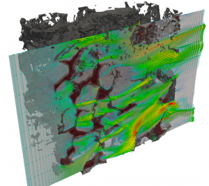
TransAT© is a versatile fluid-flow simulation platform (CFD/CMFD) using the Immersed Surfaces Technology for multi-dimensional meshing
The platform is particularly suitable for multiphase flows using tailored predictive techniques augmented by a wide-range of models accounting for complex physics
TransAT can be deployed under Linux and Windows operating systems, and is parallelized using MPI parallel protocol for HPC infinite-band systems
TransAT can be employed in various engineering verticals, including oil & gas, energy systems, chemical and process engineering, hydraulics and waste water, transportation and environment
Core Features

Immersed surfaces meshing
Transorming stl CAD files into solid level-set functions immersed into Cartesian grids with block refinement
")
Basic model portfolio
RANS and LES/V-LES approaches, convective-radiative heat transfer, reactive flows, mass transfer

All-speed formulation
Handling both incompressible & compressible flows, with possible extention to multiphase flows

Embedded sources modelling
Embedded mass, momentum and heat sources, including jets, rotating fans, fire and smoke spots

Rigid body motion
Supports using UDF the specification of motion to solid objects for up to six DOF without re-meshing
Advanced model portfolio
Porous media, combustion, visco-elasticity, shear thinning, flocculation, ozonation, erosion, miscibility

Scalable HPC
High MPI-based parallel efficiency breaking up the 95% scaling up to 10K cores & 15K cells per core

Comprehensive UDF framework
A set of UDFs for most of the single- & multiphase physics, with a comprehensive template library

State-of-the-art features
Axisymmetry, swirling & buoyancy, rotating frame of reference, advanced initial conditions, periodicity
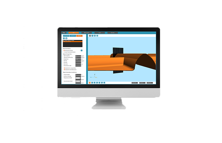
Download TransAT - get started
The new desktop version of TransAT Suite – with the modules HPC, Multiphase and Multiphysics- is now available for download. The in-built demo license allows running simulations for 1 hour using maximum 4 processors
Login and Download
Multiphase Features

Fluid-fluid interfaces

Particle & droplets flows

Gas-liquid mixtures

Granular flows

N-Phase Systems

Boiling & condensation
Advanced Physics

Gas hydrates
")
Bedload transport

Interphase mass transfer

Viscoelastic multiphase flows

Erosion
")


